Introduction
The Fast Fourier Transform (FFT) is an implementation of the Discrete Fourier Transform (DFT) using a divide-and-conquer approach. A DFT can transform any discrete signal, such as an image, to and from the frequency domain. Once in the frequency domain, many effects that are generally expensive in the image domain become trivial and inexpensive. The transformations between the image domain and frequency domain can incur significant overhead. This sample demonstrates an optimized FFT that uses compute shaders and Shared Local Memory (SLM) to improve performance by reducing memory bandwidth.
Two techniques for performing the FFT will be discussed in this sample. The first technique is called the UAV technique and operates by ping-ponging data repeatedly between Unordered Access Views (UAVs). The second technique, the SLM (Shared Local Memory) technique, is a more memory-bandwidth-efficient method, showing significant performance gains when bottlenecked by memory bandwidth.
The previous sample, Implementation of Fast Fourier Transform for Image Processing in DirectX 10, implements the UAV technique using pixel shaders. Refer to that sample for more information regarding the UAV technique and the FFT algorithm in general.
UAV Technique
The UAV technique, as described in the original sample, performs passes, commonly known as butterfly passes. Each pass requires sampling each of the real and imaginary input textures two full times and writing to the output real and complex textures once. Depending on cache architecture, this can result in performance problems caused by cache thrashing. Figure 1 shows the dispatch calls required by the UAV technique.
June 5th: The AI Audit in NYC
Join us next week in NYC to engage with top executive leaders, delving into strategies for auditing AI models to ensure fairness, optimal performance, and ethical compliance across diverse organizations. Secure your attendance for this exclusive invite-only event.
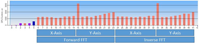
Figure 1: Compute shader dispatch calls using the UAV technique captured in Graphics Performance Analyzer (GPA)
SLM Technique
The SLM technique uses a single dispatch for each FFT axis pass. It dispatches a thread group for each row in the texture, and each thread group creates a thread for each column in the texture. Each row is represented by a thread group, and each pixel within that row is processed by a single thread. Each thread performs all butterfly passes for its respective pixel. Because of the dependency between passes, all threads within a thread group must complete each pass before any thread can move on to the next. Figure 2 shows the workflow of a thread group.
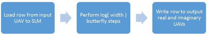
Figure 2: Thread group workflow. A thread group is created for each row in the input texture
The GroupMemoryBarrierWithGroupSync function can be used after each thread performs a butterfly pass to enforce this synchronization.
The results of each pass are stored in alternating indices in a SLM array. The source texture’s input values are initially loaded into the first half of the array and each subsequent pass writes values to the other half. Essentially, the ping ponging between textures used in the UAV technique still occurs but is done within SLM.
The operations done on each thread for each pass include:
- Calculate 2 indices for indexing into the previous pass’s output.
- Calculate 2 weights for scaling the values at each index.
- Perform basic arithmetic using indices and weights and write the result to the other side of the SLM array.
- Call GroupMemoryBarrierWithGroupSync to synchronize with other thread.
- Repeat.
The described operations are represented in the compute shader code in Figure 3. Figure 4 shows the dispatch calls required for the SLM technique.
01 |
groupshared float3 pingPongArray[4][LENGTH]; |
02 |
void ButterflyPass(int passIndex, uint x, uint t0, uint t1, out float3 resultR, out float3 resultI) |
06 |
GetButterflyValues( passIndex, x, Indices, Weights ); |
08 |
float3 inputR1 = pingPongArray[t0][Indices.x]; |
09 |
float3 inputI1 = pingPongArray[t1][Indices.x]; |
11 |
float3 inputR2 = pingPongArray[t0][Indices.y]; |
12 |
float3 inputI2 = pingPongArray[t1][Indices.y]; |
14 |
resultR = inputR1 + Weights.x * inputR2 - Weights.y * inputI2; |
15 |
resultI = inputI1 + Weights.y * inputR2 + Weights.x * inputI2; |
18 |
[numthreads( WIDTH, 1, 1 )] |
19 |
void ButterflySLM(uint3 position : SV_DispatchThreadID) |
22 |
pingPongArray[0][position.x].xyz = TextureSourceR[position]; |
23 |
pingPongArray[1][position.x].xyz = TextureSourceI[position]; |
25 |
uint4 textureIndices = uint4(0, 1, 2, 3); |
27 |
for( int i = 0; i < BUTTERFLY_COUNT-1; i++ ) |
29 |
GroupMemoryBarrierWithGroupSync(); |
30 |
ButterflyPass( i, position.x, textureIndices.x, textureIndices.y, |
31 |
pingPongArray[textureIndices.z][position.x].xyz, |
32 |
pingPongArray[textureIndices.w][position.x].xyz ); |
33 |
textureIndices.xyzw = textureIndices.zwxy; |
37 |
GroupMemoryBarrierWithGroupSync(); |
38 |
ButterflyPass(BUTTERFLY_COUNT - 1, position.x, textureIndices.x, textureIndices.y, TextureTargetR[position], TextureTargetI[position]); |
Figure 3: SLM technique implementation
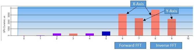
Figure 4: Compute shader dispatch calls using the SLM technique captured in Graphics Performance Analyzer (GPA)
With minor modification, the algorithm can be transposed to be performed on the y-axis as well.
Memory Bandwidth Analysis
Each color component of an image in the frequency domain is represented using a real and a complex(imaginary) plane. These planes require high precision and therefore use 128-bit R32G32B32A32.
The formulas in Figure 5 can be used to compute memory bandwidth for an FFT on the x-axis using the UAV technique. BytesRead is multiplied by 2 twice because each butterfly pass requires 4 texture samples, 2 real and 2 imaginary.
1 |
TextureSize = Width * Height * 16 |
2 |
PassCount = log2(Width) |
3 |
BytesRead = TextureSize * PassCount * 2 * 2 |
4 |
BytesWritten = TextureSize * PassCount * 2 |
Figure 5: Memory bandwidth for UAV technique
Using these formulas Figure 6 shows the calculations for the memory bandwidth of a 512×256 texture to be:
1 |
TextureSize = 512 * 256 * 16 = 2097152 |
2 |
PassCount = log2(512) = 9 |
3 |
BytesRead = 2097152 * 9 * 2 * 2 = 75497472 |
4 |
BytesWritten = 2097152 * 9 * 2 = 37748736 |
Figure 6: Memory bandwidth for a 512×256 texture using the UAV technique
That is, for just the x-axis pass, 72MB of texture reads and 32MB of texture writes are required. The y-axis transform and the inverse transforms will further increase memory bandwidth.
The SLM technique reduces memory bandwidth by taking advantage of the fact that each row can be processed independently. The technique uses compute shaders to read an entire row into shared local memory, perform all butterfly passes, and then write the results a single time to the output textures.
Figure 7 shows the simple formulas for calculating memory bandwidth of the SLM technique; they read and write each texture once and are unaffected by the pass count.
1 |
TextureSize = Width * Height * 4 |
2 |
BytesRead = TextureSize * 2 |
3 |
BytesWritten = TextureSize * 2 |
Figure 7: Memory bandwidth using the SLM technique
1 |
TextureSize = 512 * 256 * 16 = 2097152 |
2 |
BytesRead = 2097152 * 2 = 4194304 |
3 |
BytesWritten = 2097152 * 2 = 4194304 |
Figure 8: Memory bandwidth for a 512×256 texture using the SLM technique
The 4MB read and write bandwidth calculated in Figure 8 can be further improved by avoiding the initial read of the imaginary texture as it will always be zero. That makes the read bandwidth 2MB and write bandwidth 4MB. For the x-axis FFT transform the SLM technique reduces the read and write bandwidth by a factor of 36 and 8 respectively.
Using a butterfly lookup texture with pre-calculated weights and indices further increases bandwidth. The look up texture stores 2 indices and 2 weights in an R32G32B32A32 format. Each thread group will consume the entire texture over the course of all the butterfly passes, and there is a thread group for each row in the source texture. Figure 9 shows the formulas for using a butterfly look-up texture when transforming a 512×256 texture. The result is approximately 18MB of additional texture reads (Figure 10).
1 |
PassCount = log2(Width) |
2 |
ButterflyTextureSize = Width * PassCount * 16 |
3 |
BytesRead = ButterflyTextureSize * Height |
Figure 9: Generic formulas for calculating memory bandwidth of using a butterfly lookup texture
1 |
PassCount = log2(512) = 9 |
2 |
ButterflyTextureSize = 512 * 9 * 16 = 73728 |
3 |
BytesRead = 73728 * 256 = 18874368 |
Figure 10: Additional memory bandwidth requirement for using a butterfly lookup texture on a 512×256 source texture
The calculations in this section estimate the ideal memory bandwidth without accounting for additional reads that occur when partial writes are performed. These reads can be significant and will vary depending on hardware implementation.
Butterfly Lookup Texture
The calculation of the indices and weights to use on each pass for each pixel can be pre-calculated and stored in a texture. Using a butterfly texture reduces computations, but significantly increases memory bandwidth. After applying each butterfly, each row will essentially have sampled the entire 128-bit butterfly texture. Depending on the GPU architecture, using a butterfly texture may actually decrease performance as demonstrated in Figure 11.
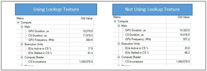
Figure 11: Results of running Graphics Performance Analyzer (GPA) on an Intel® Core™ i5-4300U processor show decreased compute shader stalling, memory reads, and duration.
Figure 12 shows a function to calculate the butterfly indices and weights in HLSL given a pass index and an offset.
01 |
void GetButterflyValues( uint passIndex, uint x, out uint2 indices, out float2 weights ) |
03 |
int sectionWidth = 2 << passIndex; |
04 |
int halfSectionWidth = sectionWidth / 2; |
06 |
int sectionStartOffset = x & ~(sectionWidth - 1); |
07 |
int halfSectionOffset = x & (halfSectionWidth - 1); |
08 |
int sectionOffset = x & (sectionWidth - 1); |
10 |
sincos( 2.0*PI*sectionOffset / (float)sectionWidth, weights.y, weights.x ); |
11 |
weights.y = -weights.y; |
13 |
indices.x = sectionStartOffset + halfSectionOffset; |
14 |
indices.y = sectionStartOffset + halfSectionOffset + halfSectionWidth; |
18 |
indices = reversebits(indices) >> (32 - BUTTERFLY_COUNT) & (LENGTH - 1); |
Figure 12: Calculating the butterfly indices and weights in a compute shader
Performance
The SLM technique shows a considerable performance advantage over the UAV technique across multiple GPUs from both Intel® and AMD*. Figure 13 shows the transformation times of a 512×512 texture to and from the frequency domain with various configuration.
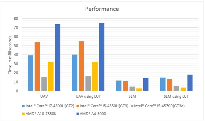
Figure 13: Combined time in milliseconds for forward and inverse transforms on both axes1
Further Optimizations
A few other optimizations became apparent in the process of writing this sample but were left out for simplicity.
Packing Components
One additional optimization would be to pack the UAV data to remove the unused alpha channel. Unfortunately, the texture format UAVs is restricted, and a 3 component 32-bit precision texture (R32G32B32) is not supported. However, the real and imaginary planes could be packed into one R32G32B32A32 texture and one R32B32 texture. You could store all components of the real number in the RGB of the first texture, and split the imaginary components up so that one component is in the alpha component of the ARGB texture and the other two components are in the R32B32.
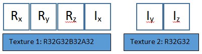
Figure 14: Example of packing the real and imaginary values into an R32G32B32A32 texture and an R32G32 texture
Avoid Unnecessarily High Precision Textures
To simplify the sample, the input image is copied into the real R32G32B32A32 texture before transforming. The inverse transform also outputs to that same texture format. Reading directly from the source texture without the copy would reduce memory bandwidth. The inverted result could also be written to a lower precision texture format.
Conclusion
Using SLM for scratch memory in an FFT algorithm yielded a substantial performance gain on the integrated GPUs analyzed. You should consider using SLM for any memory-bound, multi-pass algorithm that stores temporary data in textures. Performance on other GPUs can be analyzed using the sample code to determine which technique is most appropriate. Because of the similarities of the two techniques, supporting both should require minimal code changes.
1Software and workloads used in performance tests may have been optimized for performance only on Intel microprocessors. Performance tests, such as SYSmark* and MobileMark*, are measured using specific computer systems, components, software, operations, and functions. Any change to any of those factors may cause the results to vary. You should consult other information and performance tests to assist you in fully evaluating your contemplated purchases, including the performance of that product when combined with other products.
Configurations: For more information go to http://www.intel.com/performance
By JOSEPH S. (Intel)
This story originally appeared on Software.intel.com. Copyright 2017
Daily insights on business use cases with VB Daily
If you want to impress your boss, VB Daily has you covered. We give you the inside scoop on what companies are doing with generative AI, from regulatory shifts to practical deployments, so you can share insights for maximum ROI.
Read our Privacy Policy
Thanks for subscribing. Check out more VB newsletters here.
An error occured.